Posts

Esquisse R Package

Image
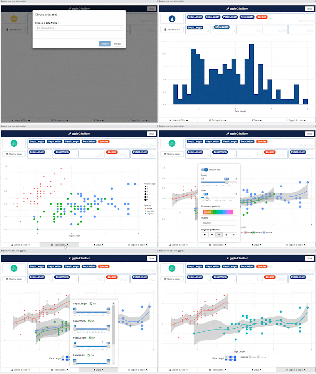
The purpose of this add-in is to let you explore your data quickly to extract the information they hold. You can only create simple plots, you won't be able to use custom scales and all the power of ggplot2. This is just the start! This addin allows you to interactively explore your data by visualizing it with the ggplot2 package. It allows you to draw bar graphs, curves, scatter plots, histograms, then export the graph or retrieve the code generating the graph. Installation Install from CRAN with : # From CRAN install.packages( " esquisse " ) Add data & drag n drop to see visual miracle.

The Multi-Armed Bandit Problem -Thompson Sampling (Ad Campaign)

Image
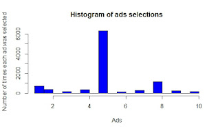
# Importing the dataset dataset = read.csv('Ads_CTR_Optimisation.csv') # Implementing Thompson Sampling N = 10000 d = 10 ads_selected = integer(0) numbers_of_rewards_1 = integer(d) numbers_of_rewards_0 = integer(d) total_reward = 0 for (n in 1:N) {   ad = 0   max_random = 0   for (i in 1:d) {     random_beta = rbeta(n = 1,                         shape1 = numbers_of_rewards_1[i] + 1,                         shape2 = numbers_of_rewards_0[i] + 1)     if (random_beta > max_random) {       max_random = random_beta       ad = i     }   }   ads_selected = append(ads_selected, ad)   reward = dataset[n, ad]   if (reward == 1) {     numbers_of_rewards_1[ad] = numbers_of_rewards_1[ad] + 1   } else {     numbers_of_rewards_0[ad] ...

The Multi-Armed Bandit Problem -Upper Confidence Bound (Ad Campaign)

Image
# Upper Confidence Bound # Importing the dataset dataset = read.csv('Ads_CTR_Optimisation.csv') # Implementing UCB N = 10000 d = 10 ads_selected = integer(0) #d is vector has only zero's numbers_of_selections = integer(d) sums_of_rewards = integer(d) total_reward = 0 for (n in 1:N) {   ad = 0   max_upper_bound = 0   for (i in 1:d) {     if (numbers_of_selections[i] > 0) {       average_reward = sums_of_rewards[i] / numbers_of_selections[i]       #upper confidence limit       delta_i = sqrt(3/2 * log(n) / numbers_of_selections[i])       upper_bound = average_reward + delta_i     } else {         upper_bound = 1e400     }     if (upper_bound > max_upper_bound) {       max_upper_bound = upper_bound       ad = i     }   }   ads_selected = append(ads_selected, ad)   ...

Eclat - A strong & stylish effect

Image
# Data Preprocessing # install.packages('arules') library(arules) dataset = read.csv('Market_Basket_Optimisation.csv') dataset = read.transactions('Market_Basket_Optimisation.csv', sep = ',', rm.duplicates = TRUE) Output distribution of transactions with duplicates: 1 5 summary(dataset) transactions as itemMatrix in sparse format with  7501 rows (elements/itemsets/transactions) and  119 columns (items) and a density of 0.03288973 most frequent items: mineral water          eggs     spaghetti  french fries     chocolate       (Other)          1788          1348          1306          1282          1229...

Apriori

Image
# Data Preprocessing # install.packages('arules') library(arules) dataset = read.csv('Market_Basket_Optimisation.csv', header = FALSE) #sparce matrix dataset = read.transactions('Market_Basket_Optimisation.csv', sep = ',', rm.duplicates = TRUE) distribution of transactions with duplicates: 1  5  summary(dataset) transactions as itemMatrix in sparse format with  7501 rows (elements/itemsets/transactions) and  119 columns (items) and a density of 0.03288973  most frequent items: mineral water          eggs     spaghetti  french fries     chocolate       (Other)           1788          1348          1306          1282          1229         22405  element (itemset/transactio...

K-Means Clustering

Image
# Importing the dataset dataset = read.csv('Mall_Customers.csv') dataset = dataset[4:5] # Splitting the dataset into the Training set and Test set # install.packages('caTools') # library(caTools) # set.seed(123) # split = sample.split(dataset$DependentVariable, SplitRatio = 0.8) # training_set = subset(dataset, split == TRUE) # test_set = subset(dataset, split == FALSE) # Feature Scaling # training_set = scale(training_set) # test_set = scale(test_set) # Using the elbow method to find the optimal number of clusters set.seed(6) wcss = vector() for (i in 1:10) wcss[i] = sum(kmeans(dataset, i)$withinss) plot(1:10,       wcss,       type = 'b',       main = paste('The Elbow Method'),       xlab = 'Number of clusters',       ylab = 'WCSS') # Fitting K-Means to the dataset set.seed(29) kmeans = kmeans(x = dataset, centers = 5) y_kmeans = kmeans$cluster # Visualising the clusters ...

Random Forest Classification

Image
# Importing the dataset dataset = read.csv('Social_Network_Ads.csv') dataset = dataset[3:5] # Encoding the target feature as factor dataset$Purchased = factor(dataset$Purchased, levels = c(0, 1)) # Splitting the dataset into the Training set and Test set # install.packages('caTools') library(caTools) set.seed(123) split = sample.split(dataset$Purchased, SplitRatio = 0.75) training_set = subset(dataset, split == TRUE) test_set = subset(dataset, split == FALSE) # Feature Scaling training_set[-3] = scale(training_set[-3]) test_set[-3] = scale(test_set[-3]) # Fitting Random Forest Classification to the Training set # install.packages('randomForest') library(randomForest) set.seed(123) classifier = randomForest(x = training_set[-3],                           y = training_set$Purchased,     ...